LOCOlib
A library for distributed \( \ell_2 \) - penalised estimation problems, implemented in Scala&Spark.
LOCOlib implements the LOCO and DUAL-LOCO algorithms for distributed statistical estimation.
Problem setting
Given a data matrix \( \mathbf{X} \in \mathbb{R}^{n\times p} \) and response \( \mathbf{y} \in \mathbb{R}^n \), LOCO is a LOw-COmmunication distributed algorithm for \( \ell_2 \) - penalised convex estimation problems of the form
\[ \min_{\boldsymbol{\beta}} J(\boldsymbol{\beta}) = \frac{1}{n} \sum_{i=1}^n f_i(\boldsymbol{\beta}^\top \mathbf{x}_i) + \frac{\lambda}{2} \Vert \boldsymbol{\beta} \Vert^2_2 \]
LOCO is suitable in a setting where the number of features \( p \) is very large so that splitting the design matrix across features rather than observations is reasonable. For instance, the number of observations \( n \) can be smaller than \( p \) or on the same order. LOCO is expected to yield good performance when the rank of the data matrix \( \boldsymbol{X} \) is much lower than the actual dimensionality of the observations \( p \).
Table of Contents
- Problem setting
- One-shot communication scheme
- Obtaining the software
- Examples
- LOCOlib options
- Preprocessing package
- Recommended Spark settings
- References
One-shot communication scheme
One large advantage of LOCO over iterative distributed algorithms such as distributed stochastic gradient descent (SGD) is that LOCO only needs one round of communication before the final results are sent back to the driver. Therefore, the communication cost – which is generally the bottleneck in distributed computing – is very low.
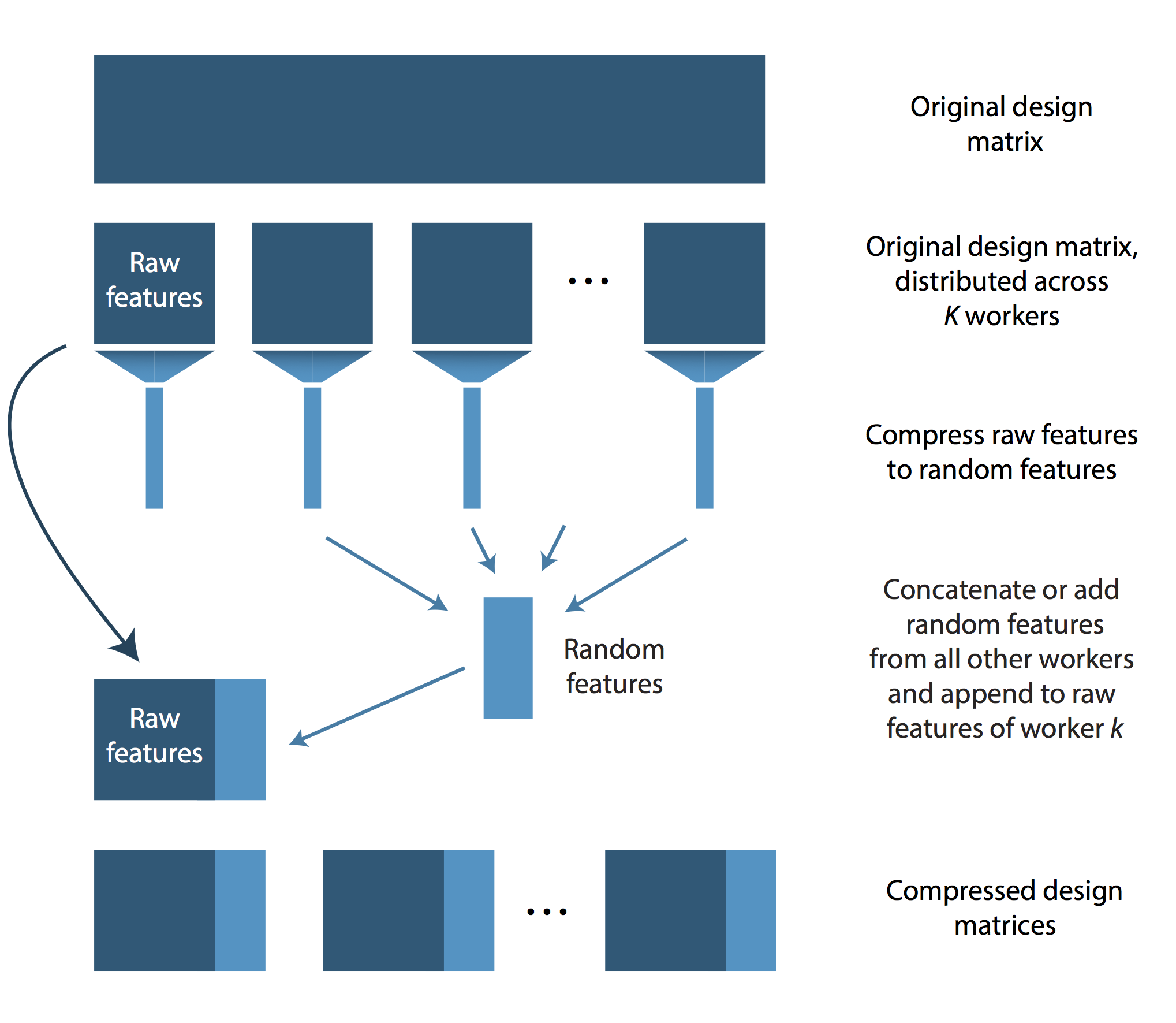
LOCO proceeds as follows. As a preprocessing step, the features need to be distributed across processing units by randomly partitioning the data into K blocks. This can be done with “preprocessingUtils” package. After this first step, some number of feature vectors are stored on each worker. We shall call these features the “raw” features of worker \(k\). Subsequently, each worker applies a dimensionality reduction on its raw features by using a random projection. The resulting features are called the “random features” of worker \(k\). Then each worker sends its random features to the other workers. Each worker then adds or concatenates the random features from the other workers and appends these random features to its own raw features. Using this scheme, each worker has access to its raw features and, additionally, to a compressed version of the remaining workers’ raw features. Using this design matrix, each worker estimates coefficients locally and returns the ones for its own raw features. As these were learned using the contribution from the random features, they approximate the optimal coefficients sufficiently well. The final estimate returned by LOCO is simply the concatenation of the raw feature coefficients returned from the \( K \) workers.
LOCO’s distribution scheme is illustrated in the following figure.
Obtaining the software
A preprocessing step is required to distribute the data across workers according to the features rather than the observations. For this step, we provide the package “preprocessingUtils”.
Building with sbt
Checkout the project repository
git clone https://github.com/christinaheinze/loco-lib.git
and build the packages with
cd loco-lib/LOCO
sbt assembly
and
cd loco-lib/preprocessingUtils
sbt assembly
To install sbt on Mac OS X using Homebrew, run brew install sbt. On Ubuntu run sudo apt-get install sbt.
Running on Windows
To run LOCO locally under Windows, we recommend using Spark 1.3.1, download winutils.exe, move it to DISK:\FOLDERS\bin\ and set HADOOP_CONF=DISK:\FOLDERS.
Examples
Ridge Regression
To run ridge regression locally on the ‘climate’ regression data set provided here, unzip climate-serialized.zip into the data directory, download a pre-build binary package of Spark, set SPARK_HOME to the location of the Spark folder, cd into loco-lib/LOCO and run:
$SPARK_HOME/bin/spark-submit \
--class "LOCO.driver" \
--master local[4] \
--driver-memory 1G \
target/scala-2.10/LOCO-assembly-0.3.0.jar \
--outdir="output" \
--saveToHDFS=false \
--readFromHDFS=false \
--nPartitions=4 \
--nExecutors=1 \
--trainingDatafile="../data/climate-serialized/climate-train-colwise/" \
--testDatafile="../data/climate-serialized/climate-test-colwise/" \
--responsePathTrain="../data/climate-serialized/climate-responseTrain.txt" \
--responsePathTest="../data/climate-serialized/climate-responseTest.txt" \
--nFeats="../data/climate-serialized/climate-nFeats.txt" \
--useSparseStructure=false \
--classification=false \
--numIterations=5000 \
--projection=SDCT \
--concatenate=false \
--CV=false \
--lambda=75 \
--nFeatsProj=389 \
--seed=3
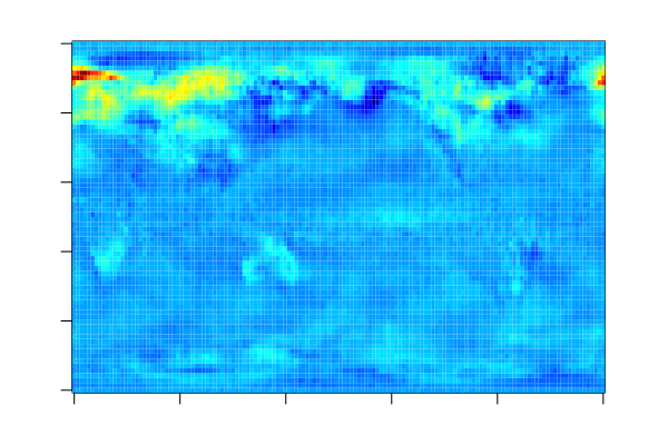
The estimated coefficients can be visualised as follows as each feature corresponds to one grid point on the globe. For more information on the data set, see LOCO: Distributing Ridge Regression with Random Projections.
SVM
To train a binary SVM with hinge loss locally on the ‘dogs vs. cats’ classification data set provided here, first preprocess the text file with the preprocessingUtils package (see below) and run:
$SPARK_HOME/bin/spark-submit \
--class "LOCO.driver" \
--master local[4] \
--driver-memory 1G \
target/scala-2.10/LOCO-assembly-0.3.0.jar \
--outdir="output" \
--saveToHDFS=false \
--readFromHDFS=false \
--nPartitions=4 \
--nExecutors=1 \
--trainingDatafile="../data/dogs_vs_cats/dogs_vs_cats_small_train-colwise/" \
--testDatafile="../data/dogs_vs_cats/dogs_vs_cats_small_test-colwise/" \
--responsePathTrain="../data/dogs_vs_cats/dogs_vs_cats_small_train-responseTrain.txt" \
--responsePathTest="../data/dogs_vs_cats/dogs_vs_cats_small_test-responseTest.txt" \
--nFeats="../data/dogs_vs_cats/dogs_vs_cats_small_train-nFeats.txt" \
--useSparseStructure=false \
--classification=true \
--numIterations=5000 \
--projection=SDCT \
--concatenate=false \
--CV=false \
--lambda=4.4 \
--nFeatsProj=200 \
--seed=2LOCOlib options
The following list provides a description of all options that can be provided to LOCO.
outdir Directory where to save the summary statistics and the estimated coefficients as text files
saveToHDFS True if output should be saved on HDFS
readFromHDFS True if preprocessing was run with saveToHDFS set to True
nPartitions Number of blocks to partition the design matrix
nExecutors Number of executors used. This information will be used to determine the tree depth in treeReduce when the random projections are added. A binary tree structure is used to minimise the memory requirements.
trainingDatafile Path to the training data files (as created by preprocessingUtils package)
testDatafile Path to the test data files (as created by preprocessingUtils package)
responsePathTrain Path to response corresponding to training data (as created by preprocessingUtils package)
responsePathTest Path to response corresponding to test data (as created by preprocessingUtils package)
nFeats Path to file containing the number of features (as created by preprocessingUtils package)
seed Random seed
useSparseStructure True if sparse data structures should be used
classification True if the problem at hand is a classification task, otherwise ridge regression will be performed
numIterations Number of iterations used in SDCA
checkDualityGap If SDCA is chosen, true if duality gap should be computed after each iteration. Note that this is a very expensive operation as it requires a pass over the full local data sets (no communication required). Should only be used for tuning purposes.
stoppingDualityGap If SDCA is chosen and checkDualityGap is set to true, duality gap at which optimisation should stop
projection Random projection to use: can be either “sparse” or “SDCT”
nFeatsProj Projection dimension
concatenate True is random projections should be concatenated, otherwise they are added. The latter is more memory efficient.
CV If true, performs cross validation
kfold Number of splits to use for cross validation
lambdaSeqFrom Start of regularisation parameter sequence to use for cross validation
lambdaSeqTo End of regularisation parameter sequence to use for cross validation
lambdaSeqBy Step size for regularisation parameter sequence to use for cross validation
lambda If no cross validation should be performed (CV=false), regularisation parameter to use
Choosing the projection dimension
The smallest possible projection dimension depends on the rank of the data matrix \( \boldsymbol{X} \). If you expect your data to be low-rank so that LOCO is suitable, we recommend using a projection dimension of about 1%-10% of the number of features you are compressing. The latter depends on whether you choose to add or to concatenate the random features. This projection dimension should be used as a starting point. Of course you can test whether your data set allows for a larger degree of compression by tuning the projection dimension together with the regularisation parameter \( \lambda \).
Concatenating the random features
As described in the original LOCO paper, the first option for collecting the random projections from the other workers is to concatenate them and append these random features to the raw features. More specifically, each worker has \( \tau = p / K \) raw features which are compressed to \( \tau_{subs} \) random features. These random features are then communicated and concatenating all random features from the remaining workers results in a dimensionality of the random features of \( (K-1) \cdot \tau_{subs} \). Finally, the full local design matrix, consisting of raw and random features, has dimension \( n \times (\tau + (K-1) \cdot \tau_{subs}) \).
Adding the random features
Alternatively one can add the random features. This is equivalent to projecting all raw features not belonging to worker \( k \) at once. If the data set is very low-rank, this scheme may allow for a smaller dimensionality of the random features than concatenation of the random features as we can now project from \( (p - p/K)\) to \( \tau_{subs} \) instead of from \( \tau = p/K \) to \( \tau_{subs} \).
Preprocessing package
The preprocessing package ‘preprocessingUtils’ can be used to
- center and/or scale the features and/or the response to have zero mean and unit variance, using Spark MLlib’s
StandardScaler. This can only be done when using a dense data structure for the features (i.e.sparsemust be set tofalse). - save data files in serialised format using the Kryo serialisation library. This code follows the example from @phatak-dev provided here.
-
convert text files of the formats “libsvm”, “comma”, and “space” (see examples under options) to object files with RDDs containing
-
observations of type
-
LabeledPoint(needed for the algorithms provided in Spark’s machine learning library MLlib) -
Array[Double]where the first entry is the response, followed by the features
-
-
feature vectors of type
-
FeatureVectorLP(needed for LOCO, see details below)
-
-
Data Structures
The preprocessing package defines a case class LOCO relies on:
FeatureVectorLP
The case class FeatureVector contains all observations of a particular variable as a vector in the field observations (can be sparse or dense). The field index serves as an identifier for the feature vector.
case class FeatureVector(index : Int, observations: org.apache.spark.mllib.linalg.Vector)Example
To use the preprocessing package
- to center and scale the features
- to split one data set into separate training and test sets
- to save the data sets as object files using Kryo serialisation, distributed over (a) observations and (b) features
download the ‘dogs vs. cats’ classification data set provided here, unzip dogs_vs_cats.zip into the data directory,
change into the corresponding directory with cd loco-lib/preprocessingUtils and run:
$SPARK_HOME/bin/spark-submit \
--class "preprocessingUtils.main" \
--master local[4] \
target/scala-2.10/preprocess-assembly-0.3.jar \
--outdir="../data/dogs_vs_cats/" \
--saveToHDFS=false \
--nPartitions=4 \
--dataFormat=text \
--sparse=false \
--textDataFormat=spaces \
--separateTrainTestFiles=false \
--proportionTest=0.2 \
--dataFile="../data/dogs_vs_cats_n5000.txt" \
--centerFeatures=true \
--scaleFeatures=true \
--centerResponse=false \
--scaleResponse=false \
--outputTrainFileName="dogs_vs_cats_small_train" \
--outputTestFileName="dogs_vs_cats_small_test" \
--twoOutputClasses=false \
--seed=1
preprocessingUtils options
The following list provides a description of all options that can be provided to the package ‘preprocessingUtils’.
outdir Directory where to save the converted data files
saveToHDFS True if output should be saved on HDFS
nPartitions Number of partitions to use
dataFormat Can be either “text” or “object”
sparse True if sparse data structures should be used
textDataFormat If dataFormat is “text”, it can have the following formats:
- “libsvm” : LIBSVM format, e.g.:
0 1:1.2 2:3.1 ...
1 1:-2.1 2:4.3 ...- “comma” : The response is separated by a comma from the features. The features are separated by spaces, e.g.:
0, 1.2 3.1 ...
1, -2.1 4.3 ...- “spaces” : Both the response and the features are separated by spaces, e.g.:
0 1.2 3.1 ...
1 -2.1 4.3 ...
dataFile Path to the input data file
separateTrainTestFiles True if (input) training and test set are provided in different files
trainingDatafile If training and test set are provided in different files, path to the training data file
testDatafile If training and test set are provided in different files, path to the test data file
proportionTest If training and test set are not provided separately, proportion of data set to use for testing
seed Random seed
outputTrainFileName File name for folder containing the training data
outputTestFileName File name for folder containing the test data
outputClass Specifies the type of the elements in the output RDDs : can be LabeledPoint or DoubleArray
twoOutputClasses True if same training/test pair should be saved in two different formats
secondOutputClass If twoOutputClasses is true, specifies the type of the elements in the corresponding output RDDs
centerFeatures True if features should be centred to have zero mean
centerResponse True if response should be centred to have zero mean
scaleFeatures True if features should be scaled to have unit variance
scaleResponse True if response should be scaled to have unit variance
Recommended Spark settings
Note that the benefit of some of these setting highly depends on the particular architecture you will be using, i.e. we cannot guarantee that they will yield optimal performance of LOCO.
- Use Kryo serialisation
--conf "spark.serializer=org.apache.spark.serializer.KryoSerializer" - Increase the maximum allowable size of the Kryo serialization buffer
--conf "spark.kryoserializer.buffer.max=1024m" - Use Java’s more recent “garbage first” garbage collector which was designed for heaps larger than 4GB if there are no memory constraints
--conf "spark.executor.extraJavaOptions=-XX:+UseG1GC"- Set the total size of serialised results of all partitions large enough to allow for the random projections to be send to the driver
--conf "spark.driver.maxResultSize=3g" References
The LOCO algorithm is described in the following papers:
- Heinze, C., McWilliams, B., Meinshausen, N., Krummenacher, G., Vanchinathan, H. P. (2015) LOCO: Distributing Ridge Regression with Random Projections
- Heinze, C., McWilliams, B., Meinshausen, N. DUAL-LOCO: Distributing Statistical Estimation Using Random Projections AISTATS 2016
Further references:
- Shalev-Shwartz, S. and Zhang, T. Stochastic dual coordinate ascent methods for regularized loss minimization. JMLR, 14:567–599, February 2013c.